
Adding alternating blank lines in Excel will support adding content to the data table. Normally you can also use the add row feature in Excel, but if you do this, it takes a lot of time and is quite manual. The article below will show you some ways to add alternating blank lines in Excel.
How to insert alternating blank lines in Excel using Go to Special
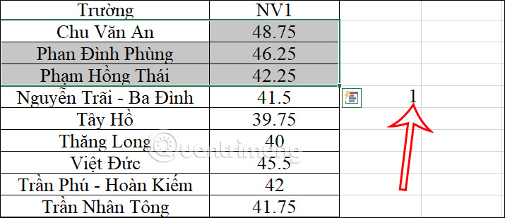
With this data table, we will insert 1 blank line alternating with 3 data lines to use as a Field header line, for example.

Step 1:
In the extra column outside the data table, in the 4th line we will fill in the number 1, meaning inserting a blank line after 3 lines of data.
Step 2:
Next From cell number 1, select 2 new cells again.
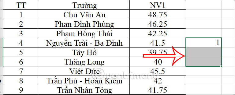
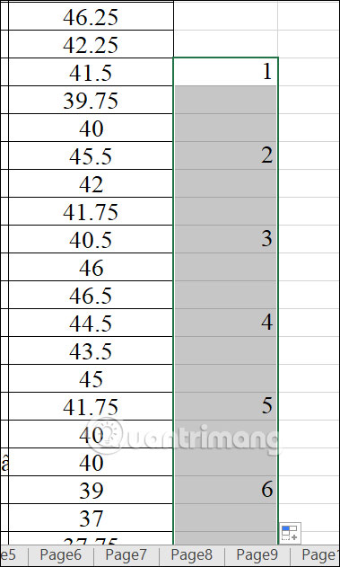
Then at the bottom right corner of the new square add 2 lines, we click to get the automatic sequence number column. The result is as shown below.
Step 3:
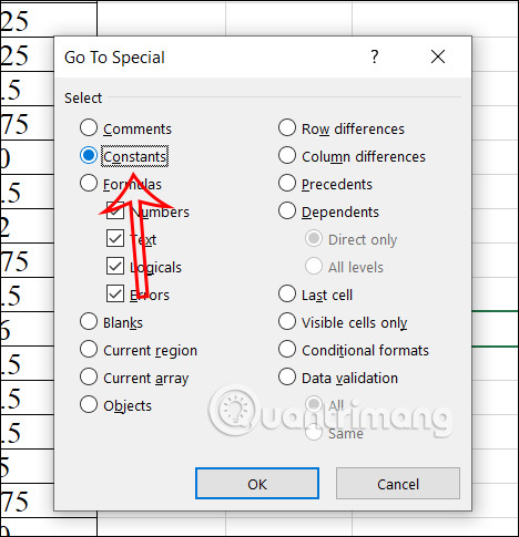
You press Key combination Ctrl + G to open the Go To dialog box and then click next Special button.
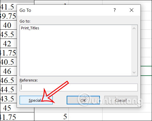
In the new dialog box that appears, click item Constants then click OK below.
Step 4:
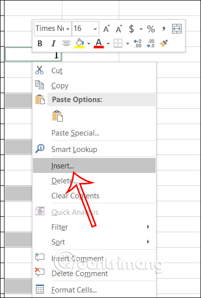
Continue, right-click on this column select Insert in the displayed list.
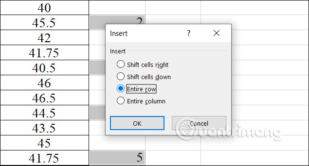
Click Entire Row section then click OK below.
Step 5:
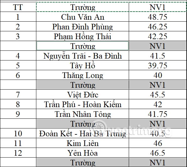
As a result, you see that every 3 lines of data there is an alternating blank line for you to use. Now you just need to fill in the title for the alternating blank lines in the data table.

Step 6:
To Quickly fill in the subject lineFriend Copy the original headline Already Black out the entire data table and press Ctrl + G opens the Go To dialog boxclick Special.
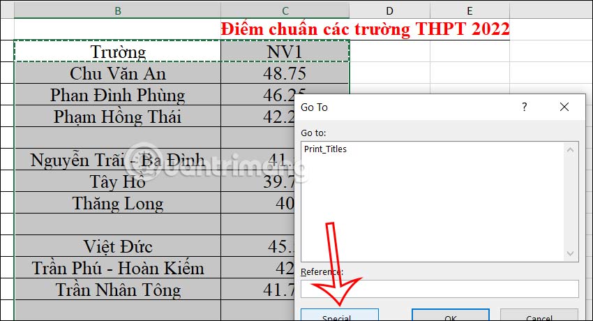
Select Blanks to select only blank rows in the selected data area.
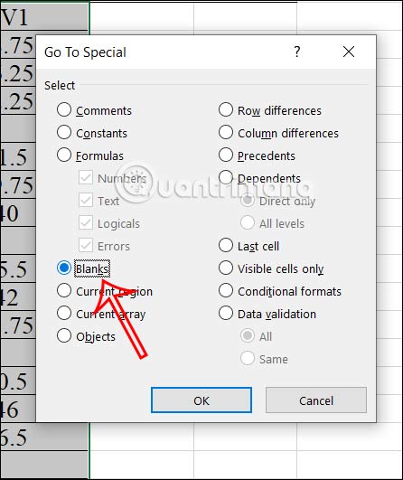
Finally we Paste the title line in the Excel table okay.

The results are in the data table as shown below.
Video tutorial on alternating blank lines in Excel
How to insert blank lines alternately in Excel using Sort
Step 1:
Open the Excel file and need to add alternating white lines in the content. First, add to the last column of the data table the serial number from 1 to the end and repeat on the lines below that do not have data.

To operate faster, enter number 1 then press and hold Ctrl then drag the mouse to the right corner and drag it down below.

Step 2:
Next, at the serial number line added below, right-click and select Sort and choose Custom Sort.

Step 3:
A small window interface appears Sort Warning. We continue to click the button Sort right below. Noteselect Expand the selection.

Step 4:
In the interface Sort new, Uncheck My data has header.
Next part Sort by we choose Column E. Order will be placed Smallest to Largest from smallest to largest. Then press OK.

The final result will appear an additional white line in the Excel data table content as shown below. We just need to delete the serial number in column E and we're done.

Noteif you want to add 2 or 3 blank lines to the table, you also need to create a number from 1 to the line you want to insert, then if you want to insert 2 or 3 lines, repeat the corresponding number.
As shown below, I will create 2 additional alternating white lines in the table, creating 2 more columns from 1 to 3.

Then, perform the same steps as above and get the results as shown below.

So you can add one or two arbitrary blank lines to the data table. The way to do it when inserting a blank line or more than 2 blank lines in Excel is only different from adding a sequential number column from 1 to the line to be inserted.
