
Separation of Excel data in columns such as separating column data and names in Excel is essential when we make a list of students, students or other lists. When the information in the same column will affect the reading of data, information is not clear, making the data reader difficult.
The operation of separating data in Excel is relatively simple, and almost like in Excel versions. However, in Excel 2013 and above, we have more Flash fill tools to separate data in Excel box simpler and faster. Below is a guide to separating excel data in versions.
1. Instructions for separating Excel 2013, 2016, 2019
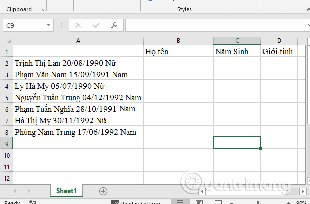
We will have the following data table with student information in the same column, and need to separate 3 separate columns including full name, year of birth and gender.
Method 1: Use the keyboard shortcut Ctrl + E for Flash Fill
Step 1:
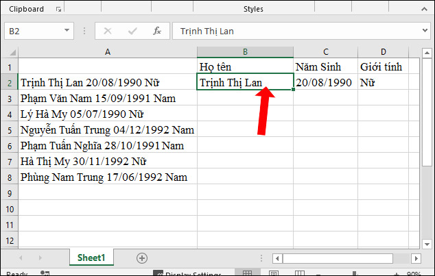
First, enter the full information for the first line in the data table.
Step 2:
Subsequent Press Enter To go down to the next box and then press Ctrl + E key combination To complete the list of remaining names in each box.
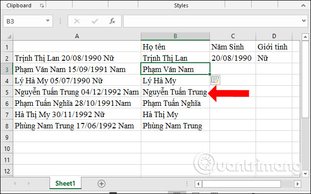
Do the same with 2 columns of birth and the other gender.
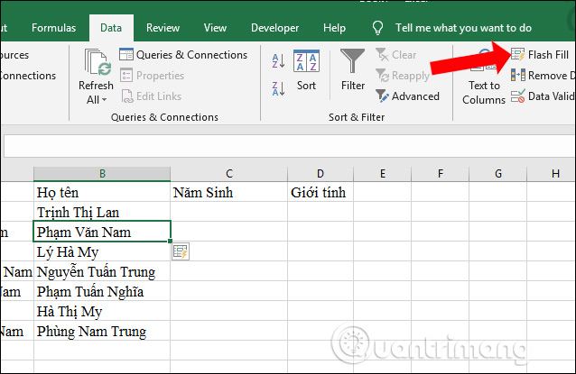
Method 2: Separate data via the Flash Fill data menu
Users also enter the information in the first cell in their full name column, then click on the second line. Tab Data On the ribbon bar Press Flash Fill To enter the corresponding values into the remaining cells in the column.
Method 3: Use a manual filling tool
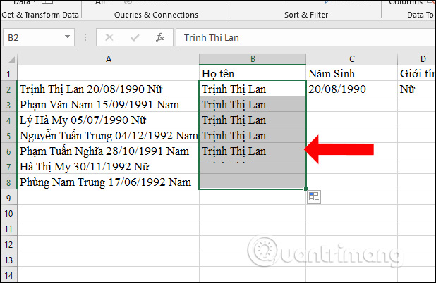
Step 1:
At the column, the username enters information for the first cell. Then hover the first cell position Show the plus sign In the lower right corner of the umbrella and pull down to the top of the column.
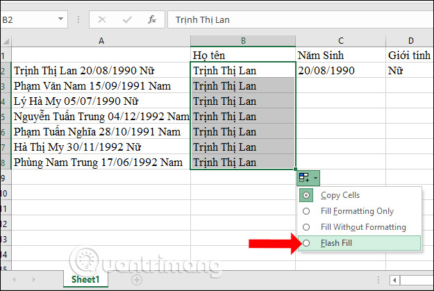
Step 2:
Then in the bottom corner of the column will display The downward triangle symbolclick and then select Flash fill In the display list.
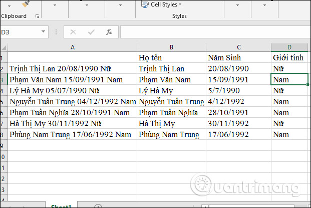
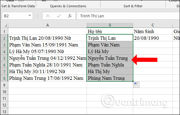
Immediately the correct values will be replaced as shown below. We perform the same operation with 2 columns of birth and gender.
Flash fill tool will only apply from word 2013 and above. With the final manual method, it will bring the corresponding index for each value of the value more effective and standard than the above two ways. If you are using the Office 2010 or below, use the text to Columns according to the instructions below.
2. How to separate data in Excel 2010, 2007 box
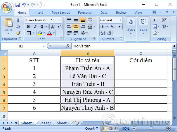
In the content table below, we will have a full column and the name attached to the score for each person. Full name is connected by the dash with the score at the same column. I will proceed to separate this column into 2 separate columns, one column is the last name and the other column is the score.
Step 1:
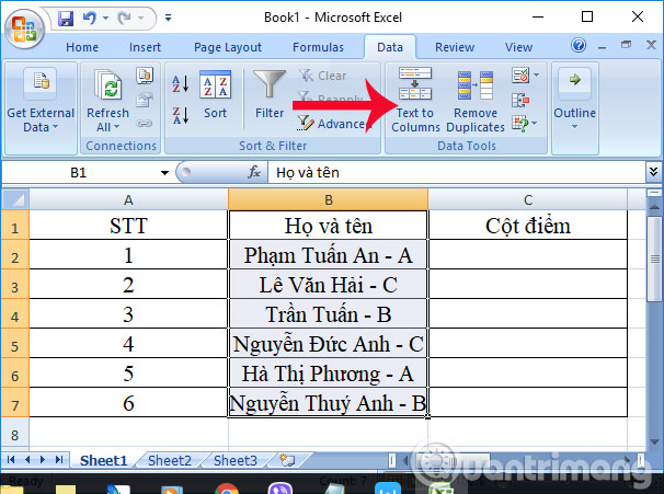
In the content of the Excel table, you need Black the content of the area to be separated into a different column. The title and the relevant content will not need to blacken. Then we click on Tab Data On the ribbon bar, then select the next item Text to Columns.
Step 2:
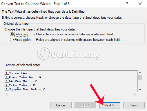
Appearing the Convert Text Text To Columns Wizard interface. Here you will need to take 3 steps to get the content column you want to separate. First of all Original Data Type There will be 2 options for separating columns, including:
- Delimited: Proceed to separate columns with separating characters such as tabs, horizontal bricks, commas, spaces …
- Fixed with: Separate the column according to the width of the data, for example, the data consists of 2 columns, although each row has different lengths, but divides the width evenly into 2 similar intervals.
In the article using horizontal bricks to separate the content, so I will select it Delimitedthen press Next At the bottom.
Step 3:
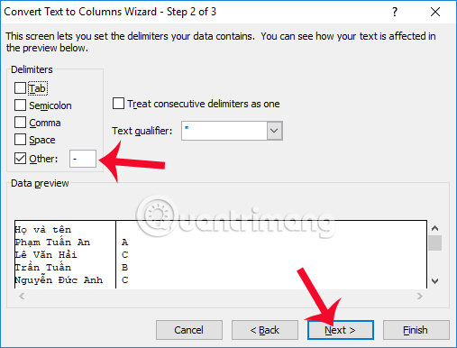
Next to the section Delimiters Select the content separation mark in the column you want to separate. There will be options including:
- Tab: Internal use is separated by a spaces of tab.
- Semicolon: A dot.
- COMMA: Use a cup with a comma.
- Space: Use a separation of spaces.
- Other: Use other parts to separate the content.
In the content due to the use of dashes to separate the content, it is advisable to click on the item Other And then fill in the dash used in the Excel file in the next box. Next, press Next To last step.
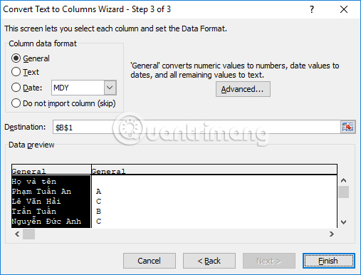
Step 4:
Shortly thereafter, you will get the results below in the Data Preview section. If you are in accordance with the requirements of separating the content in the Excel column as you like, then Excel will proceed to split into 2 separate columns. After that, you need to click on each content box to Select the format for data. For example, with the first content selected Text or General.
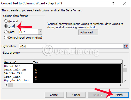
The format for the second cell is also text. Final Press Finish At the bottom to end the setting for content separation in Excel.
Step 5:
Then appear the notification board as shown below, we press OK To agree.

Thus the content in a column of the Excel table has been split into 2 columns with different content, as shown below.
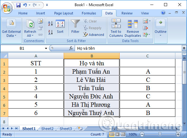
Thus, we have completed the separation of the content in the column on Excel into 2 separate columns. The operation of separating content in a column on Excel is a basic operation, often handling. This will help the content in the table easier to monitor and observe.
Video instructions for separating column content on Excel
I wish you success!
