

Network Administration – Filters are a very useful and easy-to-use feature in Microsoft Excel. With filters, you can quickly limit data to show only the necessary information. However, how to calculate the total filtered list value? The following article will help you answer the above question.
The tutorial is done on Excel 2019, but you can still apply this calculation on other versions of Excel such as Excel 2007, Excel 2010, Excel 2013, Excel 2016, because the instructions use the Excel Subtotal function.
Calculate the total filtered list value using the Subtotal function in Excel
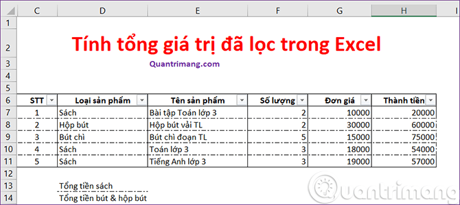
Suppose we have a data table like the following, with a filter created.
| No | Product type | Product name | Quantity | Unit price | Make money |
| 1 | Book | Math exercises for grade 3 | 2 | 10000 | 20000 |
| 2 | Pencil case | Fabric pen box TL | 2 | 30000 | 60000 |
| 3 | Pencil | Pencil section TL | 5 | 15000 | 75000 |
| 4 | Book | Grade 3 Math | 3 | 18000 | 54000 |
| 5 | Book | English grade 3 | 3 | 19000 | 57000 |
After filtering out the list of products belonging to the book category, we have the following spreadsheet:
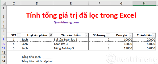
The requirement is to calculate the total cost of books. If you use the SUM() function for the above filtered data table, the result you will receive is not the total price of the book but will be the total price of all products.
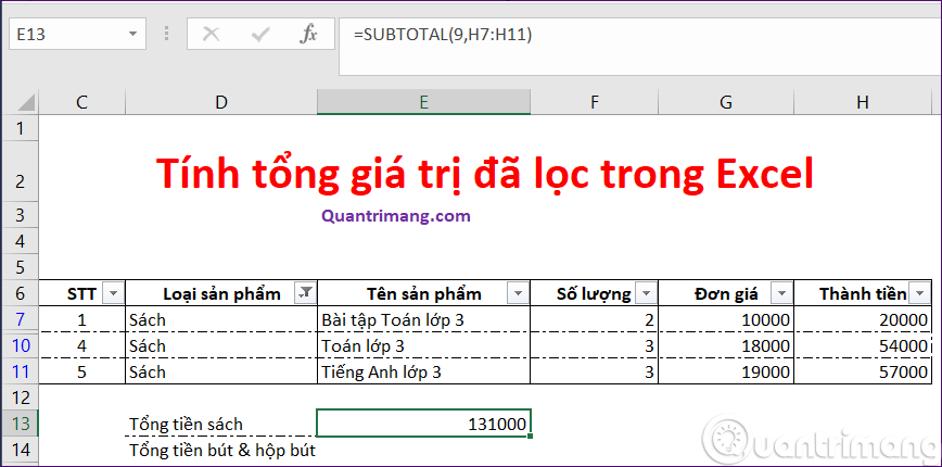
In this case, we use the SUBTOTAL function as follows. In cell E13, enter:
=SUBTOTAL(9,H7:H11)In which, 9 is the argument value corresponding to the function to use. Here we want to calculate the total, so the function to use is SUM, you can see in the table below, H7:H11 is the range to calculate the total.
The result returned the total book cost of 131,000.
About SUBTOTAL() function
The SUBTOTAL() function will look at the entire list of values in column D and calculate only those values that satisfy the filter. You can look at the image above and guess that it's because we declared argument 9. However, this argument tells Excel we want to calculate TOTAL reference values. The following table lists accepted arguments:
| Include hidden value | Ignore hidden values | Jaw |
| 1 | 101 | AVERAGE() |
| 2 | 102 | COUNT() |
| 3 | 103 | COUNTA() |
| 4 | 104 | MAX() |
| 5 | 105 | MIN() |
| 6 | 106 | PRODUCT() |
| 7 | 107 | STDEV() |
| 8 | 108 | STDEVP() |
| 9 | 109 | SUM() |
| 10 | 110 | VAR() |
| 11 | 111 | VARP() |
After looking at the table above, you are probably wondering the difference between 9 and 109. When we use the argument 9, the SUBTOTAL() function will sum the hidden values. When we use argument 109, the SUBTOTAL() function will ignore hidden values. We need to make a clear distinction hidden value and The value is eliminated because it does not satisfy the filter. Hiding a certain row can be done by right-clicking on the row order and then selecting Hide. This is completely different from rows that are not displayed because they do not satisfy the filter.
The SUBTOTAL() function is also used to perform many other useful tasks, you can refer to the tutorial on the SUBTOTAL function of Quantrimang.com.
See more:
