
COUNTIF function in Excel What is that? How to use the COUNTIF conditional counting function in Excel how? Let's find out with Quantrimang.com!
Microsoft Excel is a famous spreadsheet data processing software with many useful functions. Thanks to them, you can quickly calculate a series of data in sales tables, monthly salaries and more. Of course, to use a certain function, you need to provide data and corresponding conditions.
The COUNTIF function is a conditional counting function in Excel. You can use the COUNTIF function to count duplicate cells and count data. Below is more detailed information about COUNTIF, COUNTIF function syntax and a few illustrative examples to help you understand how to use this basic Excel function.
Table of contents of the article
What is the COUNTIF function used for?
COUNTIF is an Excel function that counts cells in a range that meet a single condition. COUNTIF can be used to count cells containing dates, numbers, and text. The criteria used in COUNTIF support logical operators (>, , =) and wildcards (*,?) for partial matching.
COUNTIF is in a group of 8 functions in Excel that divide logical criteria into two parts (range + condition). Therefore, the syntax used to construct the criteria is different, and COUNTIF requires a range of cells so you cannot use an array.
COUNTIF only supports a single condition. If you need to use multiple conditions, use the COUNTIFS function. If you need to manipulate the values in the range argument as part of a logical check, see the SUMPRODUCT and/or FILTER functions.
Syntax of the COUNTIF function in Excel
The COUNTIF function on Excel has the syntax: =COUNTIF(range;criteria)
Where range is the area where you want to count the required data. Can contain numbers, arrays, or references that contain numbers. Empty values will be ignored. Criteria is a required condition to count values in a range, which can be numbers, expressions, cell references or text strings.
Note to readers:
- The COUNTIF function returns results after using conditions with character strings of more than 255 characters.
- The criteria argument needs to be enclosed in quotes. Does not distinguish between lowercase and uppercase letters.
Question mark and star characters can be used in criteria conditions, where 1 question mark is 1 character and 1 star is 1 character string. Depending on the settings on the device, the delimiter in the function is , or ; to use.
Example of using the COUNTIF function
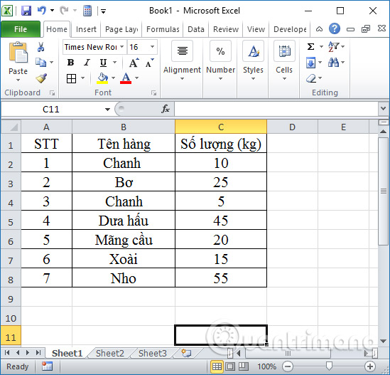
We will learn how to use the COUNTIF function with the data table below and various data search examples.
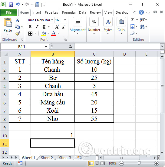
1. Search for the number of product names Mango in the table
We have a formula to do this: =COUNTIF(B2:B8,”mango”) then press Enter to execute the function.
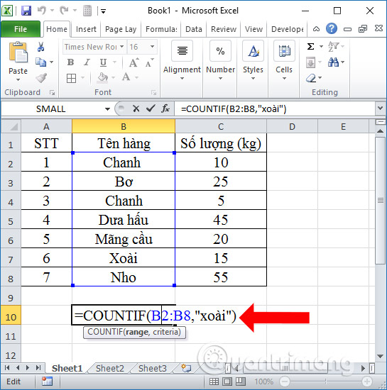
The result will be a value named Xoai in the data table.
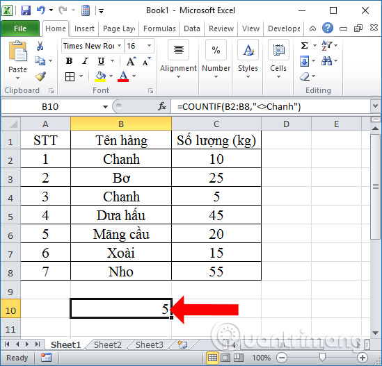
2. Find the number of rows that are not Lemons in the table
We use the condition that the row name is not Lemon “lemon” then enter the formula =COUNTIF(B2:B8,”lemon”). The result will be 5 items that do not have the name lemon in the data table.
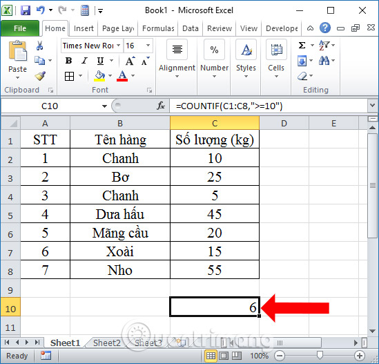
3. Find the number of items with sales quantity >= 10 kg
Terms of use with content are “>=10” in the sales quantity column with the function formula: =COUNTIF(C1:C8,”>=10″) and press Enter.
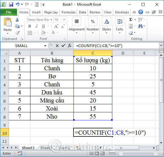
The result will be 6 items with sales quantity >= 10 kg.
4. Search for orders named Chanh using alternate characters
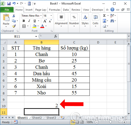
We can replace it with character * to search for values with the formula is =COUNTIF(B2:B8,”C*”) and press Enter.
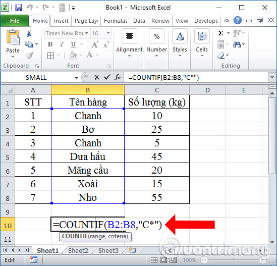
The result will be as shown below.
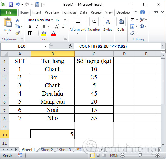
5. Search for items with names other than cell B2
Here we will find products with names other than cell B2, which is Lemon, by using the & character before the reference cell, with the function syntax =COUNTIF(B2:B8,””&B2). The result also shows the correct number of items as 5.
Combine the COUNTIF function with other functions in Excel
Use the RANK function in combination with the COUNTIF function
The RANK.EQ function can be used in conjunction with the COUNTIF function to stop skipping numbers, but will also ignore duplicate rankings.
To understand this better, let's look at how RANK.EQ works together with COUNTIF. The formula has the following form:
=RANK.EQ(B2,$B$2:$B$11,0)+COUNTIF($B$2:B2,B2)-1Implementing this formula will solve the problem of skipping numbers.
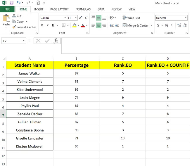
There is no overlap in the above ranks. But, James Walker and Gillian Tillmanwho were supposed to have the same rank, are now ranked differently.
Therefore, using RANK.EQ with COUNTIF solved half the problem, but it did not produce the desired results.
Use the SUMPRODUCT function with the COUNTIF function
To rank students in a list by assigning the same ranks to equivalent percentages without omitting any numbers, you can use the SUMPRODUCT function with COUNTIF.
Check out the recipe below:
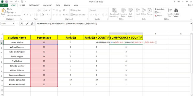
The formula may seem complicated, but it's the best way to rank items accurately. This way you can achieve the desired result, allowing for duplicate rankings and not skipping numbers.
While presenting results to your students, you can directly use the SUMPRODUCT formula as a substitute for the RANK function. To calculate unique rankings, you can use the RANK.EQ function alone or with the COUNTIF function.
Change the order of the final results
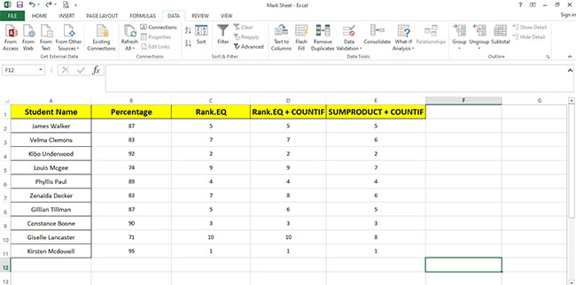
On tabs Dataclick group Sort and Filter and select ascending order to sort the rankings.
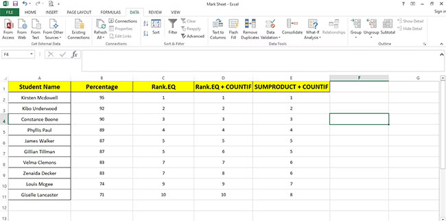
Compare the results in three rows side by side to better understand how each item ranking method works.
Common problems when using the COUNTIF function in Excel
| Problem | Solution |
| Returns false for long character strings |
The COUNTIF function returns incorrect results when you use it to match strings longer than 255 characters. To match strings longer than 255 characters, use the CONCATENATE function or operator |
| No value is returned | Be sure to enclose the criteria argument in quotes. |
| A COUNTIF formula receives a #VALUE! when referencing another worksheet | This error occurs when the formula contains functions that refer to functions that refer to cells or ranges in a workbook that are closed or cells that have been calculated. For this feature to work, you must open another workbook. |
Difference between COUNTIF and COUNTIFS functions in Excel
Both COUNTIF and COUNTIFS have the same uses. Both are used to count the number of cells that match the condition. COUNTIF is a simple function, suitable when you just need to perform a simple check. On the contrary, COUNTIFS is extremely useful when you need to check data against many conditions. See more how to use the COUNTIFS function.
It is possible to duplicate the functionality of COUNTIFS using the many AND and OR functions in COUNTIF, but it is difficult to read and compose it. COUNTIFS provides a simpler solution, helping users analyze data quickly with many conditions without needing to nest multiple levels of IF functions.
It's important to remember that COUNTIFS will check all conditions against that set of data. So, if that data matches only one of the provided sets of conditions, you should add multiple COUNTIF commands.
Overall, both COUNTIF and COUNTIFS are two Excel functions that excel at getting the necessary data out of a large group of data. You just need to use them appropriately according to each case.
Above is how to use the COUNTIF function with specific examples to use the function and how to combine characters to find values that satisfy the conditions in the data area. Note the separator , or ; It depends on each device. If you get an error in the punctuation, you need to check the separator again.
Usually, the COUNTIF function will be used with statistical data tables, asking to count the number of cells containing values that satisfy given conditions. The syntax of the COUNTIF function is quite simple, just look at it once, see the examples above from Quantrimang.com and you will definitely know how to do it.
Wishing you success!
See more:
