

COUNTIFS function in Excel There are many practical applications. Here's what you need to know about How to use the COUNTIFS function in Excel.
Microsoft Excel is a famous spreadsheet software in the world with many useful features. The advent of software makes data entry and calculating a series of numbers simpler than ever. And when using Excel, you definitely need to know it COUNTIFS function.
The COUNTIFS function in Excel is used to count cells that satisfy many given conditions. The COUNTIFS function is one of the most widely used statistical Excel functions in Excel. It is an advanced function of the COUNTIF function that only counts cells with a given condition. When working with the COUNTIFS function, users can easily find the result cells that satisfy the conditions given in the request. Conditions can be numbers, dates, text or cells containing data. The article below will guide you how to use the COUNTIFS function in Excel.
Instructions for using the COUNTIFS function in Excel
The syntax of the COUNTIFS function is =COUNTIFS(criteria_range1, criteria1, [criteria_range2, criteria2],…).
In there:
- Criteria_range1 is the first selection range that needs statistics, a required value.
- Criteria1 is a condition applied to the selection criteria_range1, the required value can be a cell, expression, or text.
- [criteria_range2, criteria2] are additional selection and condition pairs, allowing up to 127 selection and condition pairs.
Note when using the COUNTIFS function:
- Additional selections need to have the same number of rows and columns as the criteria_range1 area, and can be separate from each other.
- If the selection condition refers to an empty cell, the COUNTIFS function automatically considers the value to be 0.
- The characters ? can be used. To replace a certain character, the * sign replaces an entire string of characters. If you need to find a sign? or a real * sign, type ~ in front of that character.
- Note that the COUNTIFS function is not case sensitive.
- In general, text values need to be enclosed in quotes, but numbers do not. However, when a logical operator is included with a number, the number and the operator must be enclosed in quotes as shown below:
=COUNTIFS(A1:A10,100) // count equal to 100
=COUNTIFS(A1:A10,">50") // count greater than 50
=COUNTIFS(A1:A10,"jim") // count equal to "jim"Note: Additional conditions must follow the same rules.
- When using a value from another cell in a condition, the cell reference must be concatenated with an operator when used. In the example below, COUNTIFS will count values in A1:A10 that are less than the value in cell B1. Note that the less than operator (which is text) is enclosed in quotes, but the cell reference is not needed:
=COUNTIFS(A1:A10,"Note: COUNTIFS is one of several functions that divide a condition into two parts: Range + criteria. This causes some inconsistencies with other formulas and functions.
- COUNTIFS can count blank or non-blank cells. The formulas below count blank and non-blank cells in the range A1:A10:
=COUNTIFS(A1:A10,"") // not blank
=COUNTIFS(A1:A10,"") // blank- The easiest way to use COUNTIFS with dates is to refer to a valid date in another cell that has a cell reference. For example, to count cells in A1:A10 that contain a date greater than a date in B1, you can use a formula like this:
=COUNTIFS(A1:A10, ">"&B1) // count dates greater than A1Example of how to use the COUNTIFS function in Excel
1. Data sheet No. 1
We have the data table below to make some requests to the table.
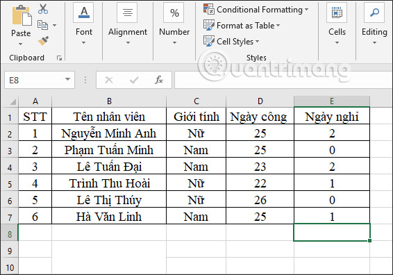
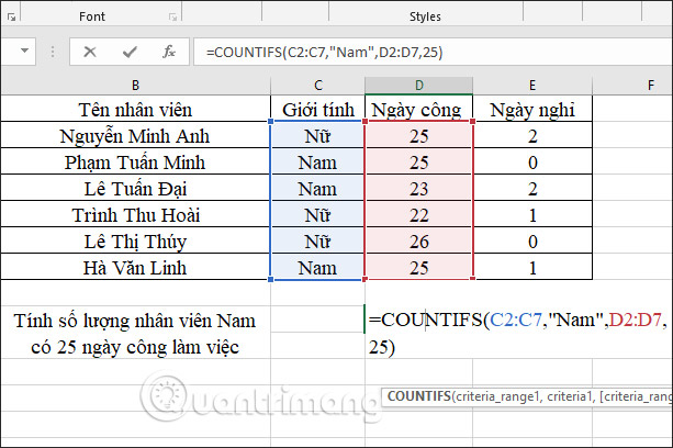
Example 1: Calculate the number of male employees with 25 working days.
In the cell where we need to enter the result, we enter the formula =COUNTIFS(C2:C7,”Male”,D2:D7,25) then press Enter.
In there:
- C2:C7 is a mandatory 1-count area with the employee's Gender.
- South is the condition of count area 1.
- C2:C7 is the 2nd count area with the employee's Workday.
- 25 is the condition of count area 2.
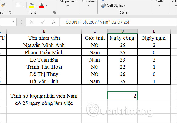
As a result, we have 2 employees, Nam, with 25 working days.
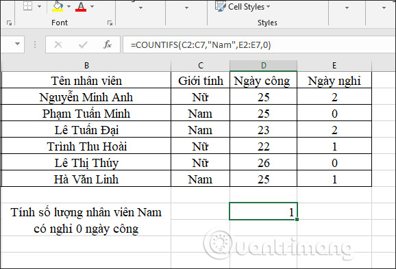
Example 2: Calculate the number of male employees whose day off is 0.
In the formula input box we enter =COUNTIFS(C2:C7,”Male”,E2:E7,0) then press Enter.
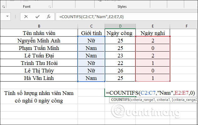
The results show 1 male employee with 0 days off.
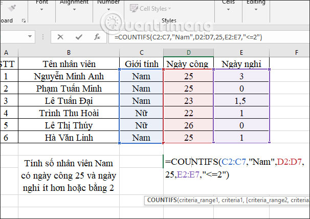
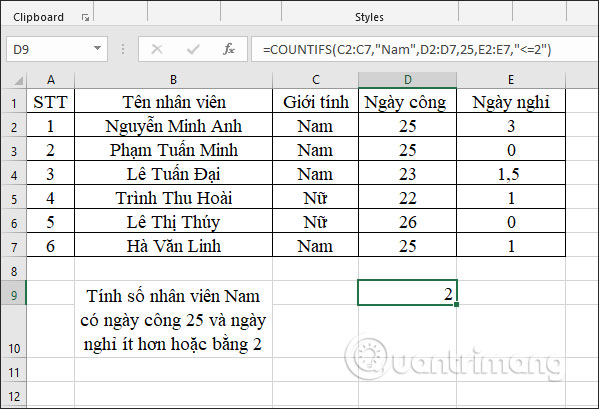
Example 3: Calculate the number of male employees who have 25 days of work and have days off less than or equal to 2 days.
We enter the formula =COUNTIFS(C2:C7,”Male”,D2:D7,25,E2:E7,” then press Enter.
As a result, there are 2 male employees who meet the requirements of having days off less than or equal to 2 days.
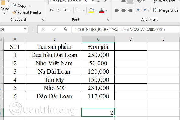
2. Data sheet number 2
Example 1: Calculate the total of Taiwanese products with a unit price of less than 200,000 VND.
In the result input box, we enter the calculation formula =COUNTIFS(B2:B7,”*Taiwan”,C2:C7,” then press Enter.
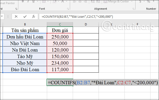
The result was 2 Taiwanese products that met the requirements.
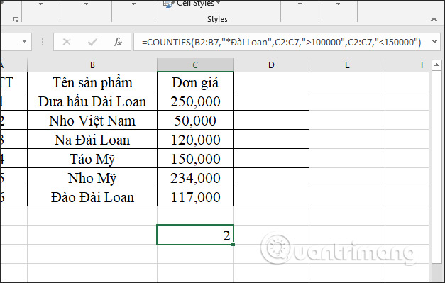
Example 2: Calculate the total Taiwanese products with unit prices between 100,000 VND and 150,000 VND.
In the result input box, we enter the formula =COUNTIFS(B2:B7,”*Taiwan”,C2:C7,”>100000″,C2:C7,” then press Enter.
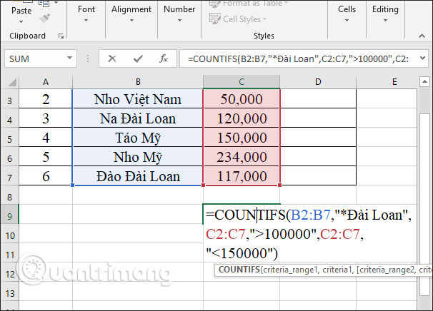
As a result, there will be 2 Taiwanese products priced between 100,000 VND – 150,000 VND.
How to use the COUNTIFS function combined with SUM in Excel
The COUNTIFS function is essentially a more complex version of the COUNTIF function. The main advantage that COUNTIFS has over COUNTIF is that it supports multiple conditions and ranges.
However, you can also define a range and a single condition for the COUNTIFS function, just like you did with the COUNTIF function.
One important thing you should understand about the COUNTIFS function before using it is that it does more than simply sum the results of the cells that meet the criteria for each cell range.
In effect, if you have two conditions for two ranges, the cells in the first range are filtered twice: Once through the first condition and then through the second condition. This means that the COUTNIFS function will only return values that meet both conditions, within their given range.
You can better understand the functionality of the COUNTIFS function by studying the example below.
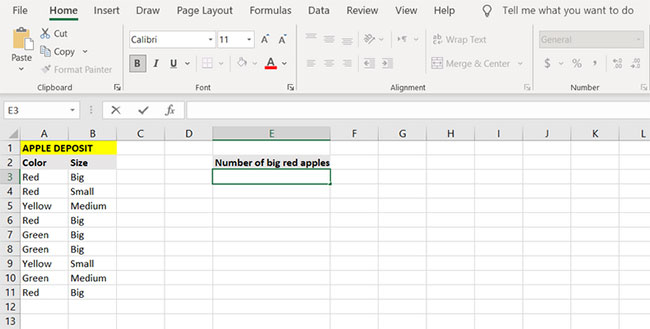
In addition to the color of the apples, there is also a column describing their size. The ultimate goal in this example is to count the number of large red apples.
1. Select the cell where you want to display the results. (In this example, the article will display the large number of red apples in cell E3).
2. Go to the formula bar and enter the formula below:
=COUNTIFS(A3:A11, "Red", B3:B11, "Big")3. With this command, the formula checks the cells from A3 arrive A11 for conditions “Red”. Cells that pass this test are then tested again within the word range B3 arrive B11 for conditions “Big”.
4. Press the button Enter.
5. Now, Excel will count the number of large red apples.
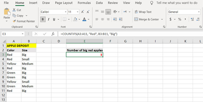
Observe how the formula counts cells that include attributes red and big. big. Formula to get cells from A3 arrive A11 and test them to find the results red. Cells that pass this condition are then again tested against the next condition in the second range, in this case, the big. big.
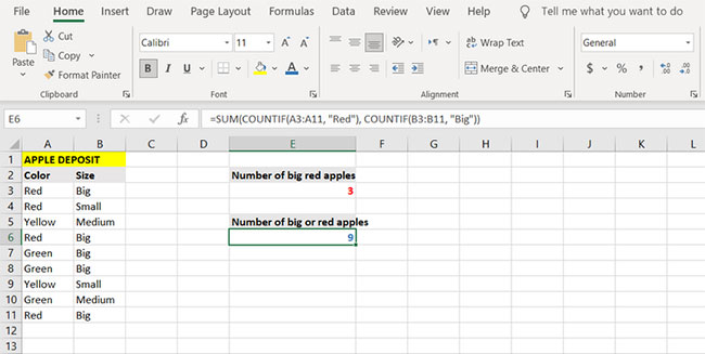
In conclusion, the ranges and conditions after the first range and condition increasingly narrow the counting filter and are not independent of each other. So, the end result of the recipe is red and big apples. You can count the number of red or large apples by combining the COUNTIF function with the SUM function.
1. Select the cell where you want to display the results of the formula. (In this example, the article will use cell E6).
2. Enter the formula below:
=SUM(COUNTIF(A3:A11, "Red"), COUNTIF(B3:B11, "Big"))3. This formula will count the cells containing red apples, then the number of cells containing large apples, and finally, it will sum these two numbers.
4. Press the button Enter.
5. Excel will now count and display the number of large or red apples.
Above are 2 data tables with usage for the COUNTIFS function in Excel. Users must write the conditions accompanying the condition data area for the COUNTIFS function to determine correctly.
How to fix common errors when using the COUNTIFS function in Excel
COUNTIFS does not work when counting text values
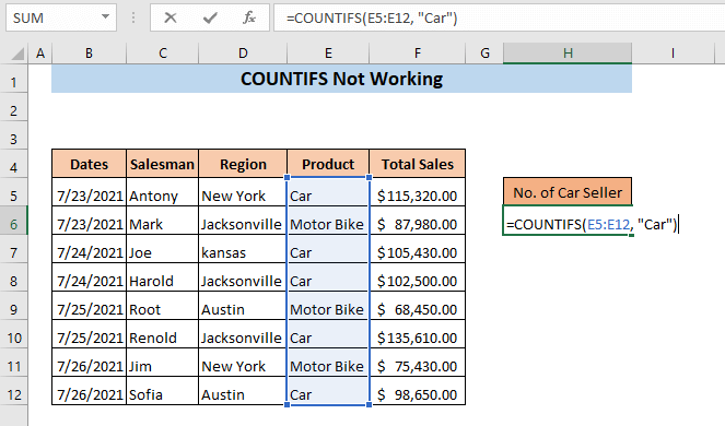
When counting text strings, they must be inserted inside quotation marks. Otherwise, the COUNTIFS function will not be able to count the text string and will return the value 0. In the following example image, the text string has not been placed in quotation marks. Therefore, this formula returns 0.
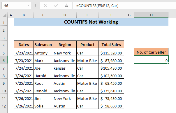
To fix this error, you just need to rewrite the formula exactly: =COUNTIFS(E5:E12, “Car”)
COUNTIFS doesn't work because the range reference is wrong
When using more than one criterion in the COUNTIFS function, the cell range for the other criteria must have the same number of cells. Otherwise, the COUNTIFS function will not work.
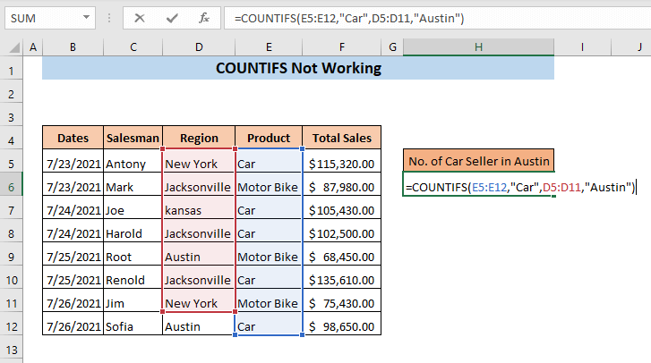
Let's say in this example we want to count car sales in Austin. The formula entered is =COUNTIFS(E5:E12,”Car”,D5:D11,”Austin”). Looking closely at the formula, you will see that the first criterion range here is E5:E12 but the second criterion range is D5:D11. The number of cells in the range for this criterion is not the same.
Now press Enterthe formula will return an error #VALUE!.
Rewrite the correct formula as follows: =COUNTIFS(E5:E12,”Car”,D5:D12,”Austin”)
COUNTIFS doesn't work because of an error in the formula
If the formula is not inserted correctly, the COUNTIFS function will not work. When using any mathematical operator, such as the greater than (>) or less than () sign, both the operator and the numeric criteria must be entered within the same equation. For example, if you want to find sales greater than $100,000, you'd insert the following formula:
=COUNTIFS(F5:F12,">" 100000)
Here, only the operator is inserted inside the equation, there is no numerical criterion.
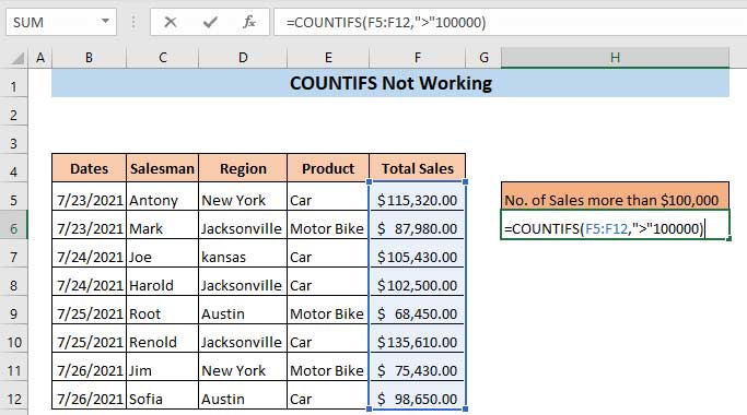
If you press Enter, the Microsoft Excel message dialog box will display: “There's a problem with this formula”.
To fix the problem. Type the exact formula:
=COUNTIFS(F5:F12,">100000")
Now we have entered both the operator and the criteria inside the parentheses. Now this formula will return the required quantity.
Press Enter.
As a result, you will receive a sales amount greater than 100,000USD.
Wishing you success!
