

SUMIF function in Excel What is that? How to use the SUMIF function how? Let's find out with Quantrimang.com!
Excel is a popular spreadsheet program from Microsoft that organizes numbers and data using functions and formulas. One of the most useful functions you should know when using Excel is the SUMIF function. You can use the SUMIF function in many different situations because this is a quite flexible Excel function. However, it can be a bit difficult for beginners. However, things to know about How to use SUMIF in Excel Below will help you get started easily.
How to use the SUMIF function in Excel
What is the SUMIF function?
SUMIF is a function used to sum values that meet certain conditions, first introduced in Excel 2007. The SUMIF function can be used to sum cells based on dates, numbers, and text that match the condition. provided conditions. This function supports logical calculations (>, , =) and symbols (*,?) to suit each part.
You may wonder, how is the SUMIF function different from the SUM function? The SUMIF function expands the capabilities of the SUM function, instead of summing within a certain range, to be totaled in SUMIF, the cells must satisfy the condition that the user passes in the criteria parameter. The SUMIF function saves a lot of effort if you want to calculate the total revenue of a unit, the sales of a group of employees, or the revenue over a certain period of time, the total salary under certain conditions…

The purpose of the SUMIF function is to sum numbers in a range that meet the provided criteria. The returned result is the sum of the provided values.
You can use the SUMIF function for financial calculations in many different contexts. Below are some good ways to use the SUMIF function in Excel.
- Calculate working hours in a certain period.
- View invoice payment deadlines.
- Track your favorite sports or soccer team stats.
- Monitor personal expenses.
- Calculate employee bonuses.
- Track page views for specific items.
SUMIF function formula
=SUMIF (range, criteria, [sum_range])
Parameters of the SUMIF function:
- Range: The range of cells you want to evaluate according to Criteria. The cells in each range must be numbers or names, arrays, or references containing numbers. Empty values and text values are ignored. The selected range can contain dates in standard Excel format.
- Criteria: Criteria for determining the values to be summed. It can be a number, an expression, or a text string.
- Sum_range: This parameter is optional, it will indicate the cells to sum. If left blank sum_rangecells within the evaluation range will be replaced.
The criteria are applied to the cells in the range. When cells in the range meet the criteria, the corresponding cells in sum_range are summed.
*Note when using the SUMIF function
The SUMIF function returns the sum of cells in a range that meet a single condition. The first argument is the range in which the criteria applies, the second argument is the criteria, and the last argument is the range containing the values to sum. SUMIF supports logical operators (>, , =) and wildcards (*,?) to match each part. Criteria can use values in another cell, as explained below.
SUMIF is in a group of 8 Excel functions that divide logical criteria into two parts (range + criteria). Therefore, the syntax used to construct the criteria is different, and SUMIF requires a range of cells for the range argument; you cannot use an array.
SUMIF only supports a single condition. If you need to apply multiple criteria, use functions SUMIFS. If you need to manipulate the values that appear in the range argument (i.e. extract the year from a date for use in criteria), see the function SUMPRODUCT and/or FILTER.
Example of how to use SUMIF in Excel
Let's learn how to use the SUMIF function with Quantrimang.com. Suppose we have a summary table of income and personal income tax as follows:
| Total income | Number of dependents | Taxable income | Personal income tax | Actual income received | Departments |
| 80,000,000 | 2 | 63,348,500 | 13,154,550 | 66,393,950 | Accountant |
| 30,000,000 | 1 | 16,948,500 | 1,792,275 | 27,756,225 | Sell |
| 20,000,000 | 1 | 6,875,000 | 437,500 | 19,037,500 | Sell |
| 10,000,000 | 1 | -3,650,000 | 0 | 8,950,000 | Sell |
| 100,000,000 | 2 | 82,750,000 | 19,112,500 | 79,837,500 | Accountant |
| 1,000,000,000 | 1 | 976,900,000 | 332,065,000 | 657,435,000 | Manager |
In Excel the table is presented as follows:

Example 1: Use the SUMIF function to calculate total personal income tax for people with income under 50 million VND.
To solve this example, we first need to determine the 3 parameters of the SUMIF function, specifically:
- Range: Column range containing total income, here is B4:B9
- Criteria To be
- Sum_range is the column range containing the personal income tax to be totaled, here is H4:H9
Then, we will have the formula: =SUMIF(B4:B9,”H4:H9)you enter this formula in the cell containing the result, in our example cell H19.

Press Enter and will receive the amount of personal income tax that needs to be paid for those with income under 50,000,0000 which is 2,229,775.

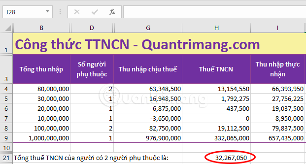
Example 2: Still with the above spreadsheet, calculate the total personal income tax of a person with 2 dependents. At this time:
- Range: The column range containing the number of dependents, here is D4:D9
- Criteria is =2, can be written as 2 or “=2”
- Sum_range is the column range containing the personal income tax to be totaled, here it is H4:H9.
Thus, the formula will be: =SUMIF(D4:D9,2,H4:H9)you enter the formula into the cell containing the result, in the example it is H21:

Press Enter to receive a total tax return of 32,267,050 VND.
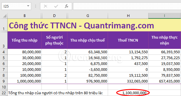
Example 3: Still in the table above, calculate the total income of people with income over 80 million VND. At this time:
- Range: Column range containing total income, here is B4:B9
- Criteria is greater than 80 million, written as “>80000000”
- Sum_range in this case is Range so you do not need to enter this parameter anymore.
So the formula will be: =SUMIF(B4:B9,”>80000000″)you enter into the cell containing the result, here is H22:

Press Enter To get the result that the total income of people with income over 80 million is 1,100,000,000:
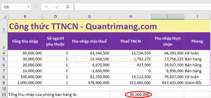
Example 4: Still using the original data table, let's calculate the total income of the sales department. Then:
- Range: The column range containing the room list here is J4:J9
- Criteria is Sales, written as “Sales”
- Sum_range is the column range containing the income to be summed, here it is B4:B9
So the formula will be: =SUMIF(J4:J9,”Sell”,B4:B9)you enter the formula into the cell containing the result, as shown below, cell H23:

Press Enter and receive a total income of 60,000,000 for the sales department:
Pay attention when using the SUMIF function
- When sum_range is omitted, the total will be calculated accordingly Range.
- Criteria containing letters or mathematical symbols must be enclosed in quotation marks “”.
- The range that defines the numeric format that can be provided as a number will not require the use of parentheses.
- Characters
?and*can all be used in Criteria. A question mark matches any single character; an asterisk matches any string of characters. If you want to find an actual question mark or asterisk, type a tilde (~) before the character.
Use Named Range
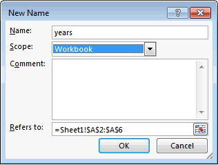
You can also use a Named Range in the SUMIF function. Named Range is a descriptive name for a set of cells or range of cells in a worksheet. If you are not sure how to set up Named Range in your spreadsheet, read Quantrimang.com's guide on: How to name Excel cells or data ranges.
For example, if you created a Named Range called years. years in your spreadsheet refer to cells A2:A6 in Sheet1 (Note that Named Range is an absolute reference to =Sheet1!$A$2:$A$6 in the image below):
The article can use this Named Range in the current example.
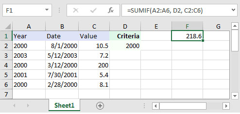
This will allow replacing A2:A6 as the first parameter with Named Range years, as follows:
=SUMIF(A2:A6, D2, C2:C6)    'First parameter uses a standard range
Result: 218.6

=SUMIF(years, D2, C2:C6)    'First parameter uses a named range called years
Result: 218.6
Some frequently asked questions
Question: I have a few cells in the worksheet, but I only need the sum of all the negative cells. So if there are 8 values, A1 to A8, and only A1, A4, and A6 are negative then I want B1 to be the sum (A1, A4, A6).
Reply: You can use the SUMIF function to sum only negative values as you described above.
For example:
=SUMIF(A1:A8,"This formula will only sum the values in cells A1:A8 – cells with negative values (i.e.:
Question: In Microsoft Excel, I am trying to achieve the following with the IF function:
If a value in any cell in column F is “food” then add the value of its corresponding cell in column G (for example, the corresponding cell for F3 is G3). The IF function is performed in another cell entirely. I can do it for a pair of cells but don't know how to do it for the entire column.
Currently, I have the following:
=IF(F3="food"; G3; 0)Reply: This formula can be created using the SUMIF function instead of using the IF function:
=SUMIF(F1:F10,"=food",G1:G10)This formula will evaluate the first 10 rows of data in the spreadsheet. You may need to adjust the ranges accordingly.
If you separate your parameters with semicolons, you may need to replace the commas in the formula above with semicolons.
Why doesn't the SUMIF formula work?
There are several reasons why the SUMIF function in Excel does not work. Sometimes your formula doesn't return the expected results just because the data type in the cell or in some of the arguments doesn't match the SUMIF function. Below are important things you need to keep in mind.
SUMIF only supports one condition
The formula of the SUMIF function only has room for one condition. To sum with multiple criteria, use the SUMIF function (add cells that meet all conditions) or build a SUMIF formula with multiple OR criteria (sum cells that meet any condition).
Range and sum_range should be the same size
For the SUMIF function formula to work correctly, the range and sum_range arguments should have the same size, otherwise you may get misleading results. The problem is that Microsoft Excel does not rely on the user's ability to provide the right range, and to avoid possible inconsistency problems, it automatically determines the total range this way:
Sum_range only identifies the upper left cell of the range to be summed. The rest is decided by the size and shape of the range argument.
Above is the basic way to use the SUMIF function in Excel. It's actually very easy, isn't it? You just need to determine the correct range of columns that need to satisfy the criteria, the criteria and the range of columns that need to be summed and you're done. If you need to calculate the sum based on many conditions, then remember to use the SUMIFS function, it's much easier and faster.
If you have any questions while working with the SUMIF function, please comment below for help.
