SUMIFS function, how to use the function to sum multiple conditions in Excel

Sumifs function in Excel Extremely useful when you have to sum multiple conditions. Here are the details How to use Sumifs function in Microsoft Excel.

The SUMIFS function in Excel is one of the basic Excel functions, a commonly used calculation function in Excel. To calculate the total in Excel, we will use the SUM function. If we want to add a certain condition to the total function, we will use the SUMIF function. In cases where the data table requires a sum with many conditions, we must use the SUMIFS function. The following article will guide you how to use the SUMIFS function in Excel.

SUMIFS function syntax in Excel

The SUMIFS function syntax in Excel has the form: =SUMIFS(sum_range,criteria_range1,criteria1,criteria_range2,criteria2,…).

In there:

• Sum_range: are the cells that need to be summed in the data table, empty values ​​and text values ​​are ignored, required parameters.
• Criteria_range1: the range that needs to be tested using the criterion criteria1, is a required value.
• Criteria1: condition applied to criteria_range1, can be a number, expression, cell reference to determine which cells in criteria_range1 will be summed, also a required value.
• Criteria_range2, criteria2,…: optional additional ranges and conditions, maximum 127 pairs of criteria_range, criteria.

Note when using the SUMIFS function in Excel

• For each cell in the range, the sum_range range will be summed when all corresponding conditions determined to be true for that cell are met.
• Cells in sum_range that contain TRUE are considered 1, cells containing FALSE are considered 0.
• Each criteria_range must have the same selection size as sum_range, criteria_range and sum_range must have the same number of rows and the same number of columns.
• Criteria can use question mark (?) characters instead of single characters or asterisks
• instead of a string. If the condition is a question mark or asterisk, you must enter a ~ sign in front, the condition value is the text enclosed in “.
• Multiple conditions are applied using AND logic, i.e. criteria1 AND criteria2, etc.
• Each additional range must have the same number of rows and columns as the total range, but the ranges do not need to be contiguous. If you provide mismatched ranges, you will get a #VALUE error.
• The text string in the criteria must be enclosed in quotation marks (“”), i.e. “apple”, “>32”, “jap*”
• Cell references in criteria must not be enclosed in quotes, i.e. “
• SUMIF and SUMIFS can handle ranges, but cannot handle arrays. This means you cannot use other functions like YEAR on the criteria range because the result is an array. If you need this functionality, use the SUMPRODUCT function.

The order of arguments between the SUMIFS and SUMIF functions is different. Sum range is the first argument in SUMIFS, but the third argument in SUMIF.

Instructions for using the SUMIFS function in Excel

Use wildcards

Wildcard characters like '*' and '?' can be used in the criteria argument when using the SUMIFS function. Using these wildcards will help you find similar but not exact matches.

Asterisk

• – It matches any string of characters, which can be used after, before or with surrounding criteria to allow partial search criteria to be used.
• For example, if you apply the following criteria in the SUMIFS function:
• N * – Implies all cells in the range starting with N

* N – Implies all cells in the range ending in N

*N* – Cells containing N

Question mark (?) – Matches any single character. Suppose you apply N?r as a criterion. “?” here will replace a single character. N?r will correspond to North, Nor, etc. However, it will not take into account Name.

What if the given data contains an asterisk or a real question mark?

In this case, you can use the tilde (~). You need to type “~” before the question mark in that case.

Use Named Ranges with the SUMIFS function

Named Range is the descriptive name of a set of cells or range of cells in a worksheet. You can use Named Ranges while using the SUMIFS function.

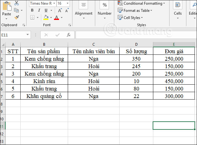
We will calculate the total with the data table below with a number of different conditions.Data table

Example 1

: Calculate the total products sold by Hoai's staff with a unit price of less than 400,000 VND.

• In the result input box, we enter the formula =SUMIFS(D2:D7,C2:C7,”Hoai”,E2:E7,”
• In there:
• D2:D7 is the area where the total item needs to be calculated.
• C2:C7 is the employee name condition value range.
• “Hoai” is the condition for the name of the employee who needs to calculate the number of items contained in area C2:C7.

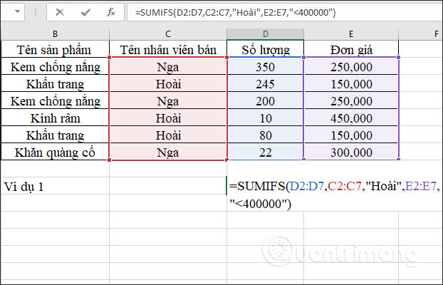
“400,000” is the condition for containing items in areas E2:E7.

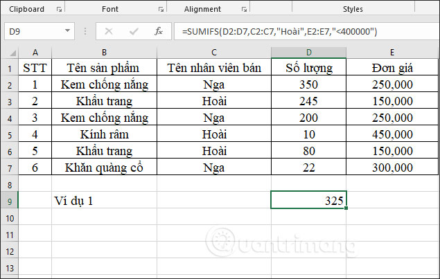
The result is the total number of items as shown below.The result is the number of products with a unit price below a certain value

Example 2

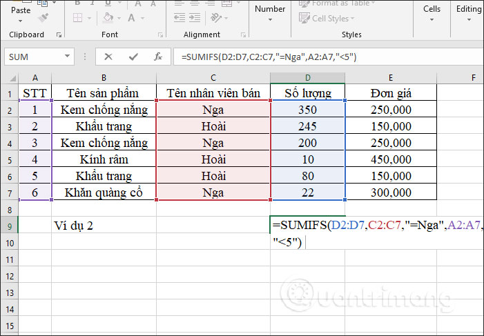
In the result input box, we enter the formula =SUMIFS(D2:D7,C2:C7,”=Nga”,A2:A7,”

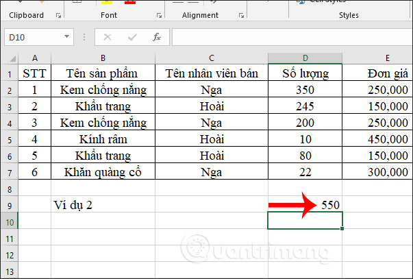
As a result, we get the total number of items sold by Russian employees with serial numbersTotal value

Example 3

In the result input box, we enter the formula =SUMIFS(D2:D7,C2:C7,“Russia”,B2:B7,“scarf”). In which the mark is used to exclude a certain object in the data area as a condition.

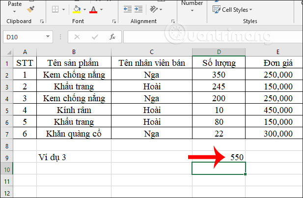
The result is the total number of products as shown below.

SUMIFS function

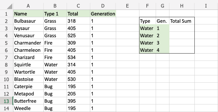
Example 4:

Calculate the total of all stats for generation 1 Water-type Pokemon:

The condition here is that Water and Generation are 1.

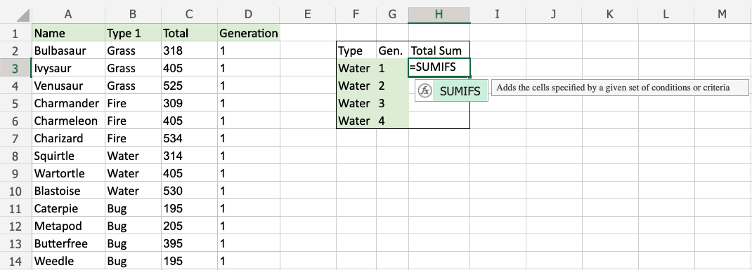
1. Here are the step-by-step details: How to use the SUMIFS function in ExcelSelect the cell
2. H3 .
3. Type =SUMIFS.
4. Double click on the command C2:C759SUMIFS.
5. Select the total range as ,
6. . B2:B759 Type
7. Select the range for the first condition F3(value type 1) WaterSelect criteria (box
8. is valuable
9. ) D2:D759 type ,
10. Select the range for the second condition from ,
11. (Generation value)
12. Type Determine the criteria (cell G3 has value 1).Press

. Results after using the SUMIFS function in Excel

Note:

You can add more conditions by repeating steps 9 through 12 before pressing Enter.

This function now calculates the sum of the total stats for generation 1 water Pokemon. This function can be repeated for future generations to compare them.

Above are some examples of how to use the SUMIFS function, calculating the total value with many combined conditions. We must arrange the ranges and accompanying conditions properly so that Excel can recognize the function formula for calculation.

• Limitations of the SUMIFS function
• The SUMIFS function has some limitations that you should be aware of:
• The conditions in SUMIFS are combined using AND logic. In other words, all conditions must be TRUE for a cell to be included in the total. To sum cells using OR logic, you can use an alternative solution in simple cases.

The SUMIFS function requires actual ranges for all range arguments; you cannot use an array. This means you can't do things like extract the year from a date inside the SUMIFS function. To change the values ​​that appear in the range argument before applying the criteria, the SUMPRODUCT function is a flexible solution.

SUMIFS is not case sensitive. To sum values ​​based on a case-sensitive condition, you can use a formula based on the SUMPRODUCT function with the EXACT function.

The most common way to work around the above limitations is to use the SUMPRODUCT function. In current versions of Excel, another option is to use the newer BYROW and BYCOL functions. How to fix #VALUE error in Excel's SUMIFS function

Problem:

The formula refers to a cell in a closed workbook

The SUMIF function that references a cell or range of cells in a closed workbook will result in a #VALUE! error.

Note: This is a common error. You also often encounter this message when using other Excel functions such as COUNTIF, COUNTIFS, COUNTBLANK…

Solution: Open the workbook contained in this formula, press F9 to refresh the formula. You can also fix the problem by using both the SUM and IF functions in an array formula.

Problem:

The criteria string is longer than 255 characters

The SUMIFS function returns wrong results when you try to combine strings longer than 255 characters.

=SUMIF(B2:B12,"long string"&"another long string")

Solution:

Shorten the string if possible. If that's not possible, use the CONCATENATE function or the & operator to split the value into multiple strings. For example:

Issue: In SUMIFS, the criteria_range argument is inconsistent with the sum_range argument. =SUMIFS(C2:C10,A2:A12,A14,B2:B12,B14) The range argument must always be the same in SUMIFS. That means the criteria_range and sum_range arguments should refer to the same number of rows and columns.

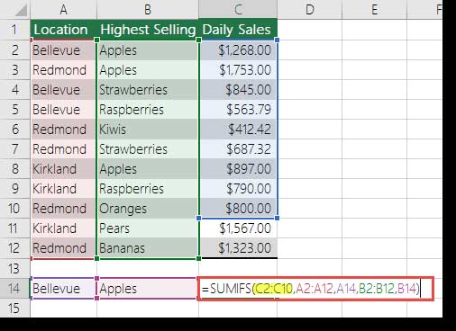
will give #VALUE error.

Example of SUMIFS function in Excel sum_range Solution:

Change